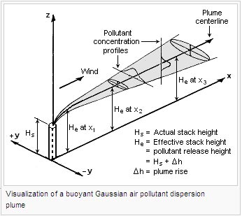
12. {\displaystyle C={\frac {\;Q}{u}}\cdot {\frac {\;f}{\sigma _{y}{\sqrt {2\pi }}}}\;\cdot {\frac {\;g_{1}+g_{2}+g_{3}}{\sigma _{z}{\sqrt {2\pi }}}}}. Eero P. Simoncelli, in The Essential Guide to Image Processing, 2009. (9.3). The Gaussian air pollutant dispersion equation (discussed above) requires the input of H (also known as the effective plume height, He) which is the pollutant plume's centerline height above ground level. #fbuilder .cff-calculated-field input{background:#d4e89a; color:black;} The distribution of price changes pt conditional on Zt=k,pt_,Zt_ is multivariate normal N[k,k. The air pollution dispersion models are also known as atmospheric dispersion models, atmospheric diffusion models, air dispersion models and air quality models. Karl B. SchnelleJr., in Encyclopedia of Physical Science and Technology (Third Edition), 2003, Algorithms based on the Gaussian model form the basis of models developed for short averaging times of 24hr or less and for long-time averages up to a year. The model generally used is as follows (Reed, 2005): X= hourly concentration at downwind distance x, g m-3, us = mean wind speed at pollutant release height, m s-1, y= standard deviation of lateral concentration distribution, z= standard deviation of vertical concentration distribution, H= pollutant release height (stack height), m, y= crosswind distance from source to receptor, m. The terms y and z are based on atmospheric stability coefficients, where larger values (usually at greater distances from the source) represent a plume with wide spread and low peak, and vice versa (Reed, 2005). Algorithms are available for single and multiple sources as well as single and multiple receptor situations. where the loading functions are known in closed form: We assume that there exist a panel of zero coupon, continuously-compounded yields Yt =[Yt,1,, Yt,k], where Yt, = log P (, rt, ) and the maturities are = 1, , n.12 In this model, if the parameters are known, the spot rate is observable from a single yield. Under the J.P. Morgan approach, the regime indicators (Zt) are assumed time independent. The European Topic Centre on Air and Climate Change, which is part of the European Environment Agency (EEA), maintains an online Model Documentation System (MDS) that includes descriptions and other information for almost all of the dispersion models developed by the countries of Europe. 9.5. To break this stochastic singularity, it is common to add an additive pricing error:13. where, for notational simplicity, we relabel Yt, as the log-bond prices, trN(0,1) is standard normal, and t N(0, ) is the vector of pricing errors. Let us also assume that V is a Gaussian random variable. Marginal models have been shown to produce better denoising results when the multiscale representation is overcomplete [20, 2730]. This technique appears to improve the performance of background modeling but still is not guaranteed to completely handle small background motions. It is more appropriate for the far field of portions of the cloud. They are thus difficult to study directly, or to utilize in deriving optimal solutions for image processing applications. To calculate V, we use the deterministic solution employing the expected value of P. This Gaussian distribution is a reasonable approximation, which does not require repetitive deterministic power flow solutions and is easy to implement. Fig. However, it is a local approximation. Given class weights wc, the distribution is. The resulting calculations for air pollutant concentrations are often expressed as an air pollutant concentration contour map in order to show the spatial variation in contaminant levels over a wide area under study. The Gaussian model specifically is well described and established [1]. Dispersion models have been validated and are well developed. Finally, r enters both in the yields and the dynamics. Once we have transformed the image to a multiscale representation, what statistical model can we use to characterize the coefficients? Before we discuss MCMC estimation, we provide a brief and informal discussion of parameter identification. Because br only appears in the yield equation, it can be difficult to generate a reasonable proposal for independence Metropolis, and thus we recommend a fat-tailed random-walk Metropolis step for br. Briggs first published his plume rise observations and comparisons in 1965. 3 Suppose, that is, we are interested in the shape of the posterior distribution. Fig. Often these methods operate by optimizing a higher-order statistic such as kurtosis (the fourth moment divided by the squared variance). These estimates show substantial improvement over the linear estimates associated with the Gaussian model of the previous section. Copyright 2021 WKC Group All Rights Reserved, About WKC Group Environmental Consultants, Sound Attenuation Calculator Inverse Square Law, Sound Attenuation Calculator Line Source, Logarithmic Addition of Sound Pressure Levels, Acoustic Induced Vibration (AIV) Screening Tool, Blast Overpressure and Grounde-Bourne Vibration Calculator, BS4142 Industrial and Commercial Sound Assessment Tool, Emissions Calculator for Engines, Turbines and Heaters, Gas Turbine Emissions Calculator US EPA AP-42, Flare Effective Height & Diameter Calculator, Correction from Actual to Normal Stack Data Calculator, Stack Gas Volumetric Flow Correction Calculator. For more information on the Gaussian dispersion model and any of the steps in this calculator, visit Lakes Environmentals online ISCST3 Tech Guide, as well as Wikipedias page on Atmospheric dispersion modeling. Copyright 2022 Elsevier B.V. or its licensors or contributors. The short-term algorithms require hourly meteorological data, while the long-term algorithms require meteorological data in a frequency distribution form. z [9], a K-means approximation is used. y Please note that this or any other calculators on the wkcgroup.com tools room are forinformation only. It controls the average long run level of the yield curve. Envir., 6:507-510, 1972, Workbook of Atmospheric Dispersion Estimates, https://citizendium.org/wiki/index.php?title=Air_pollution_dispersion_modeling&oldid=394218, Editable Main Articles with Citable Versions, Advanced Articles written in American English, Creative Commons-Attribution-ShareAlike 3.0 Unported license, Creative Commons Attribution-NonCommercial-ShareAlike, = vertical dispersion with no reflections, = vertical dispersion for reflection from the ground, = vertical dispersion for reflection from an inversion aloft. If the information regarding volatility is consistent between the spot rate evolution and yields, this approach will work well. Most regulatory air dispersion models, such as SCREEN3 and AERMOD are based on the principles of Gaussian plumedispersion. Although Briggs proposed plume rise equations for each of the above plume categories, it is important to emphasize that "the Briggs equations" which become widely used are those that he proposed for bent-over, hot buoyant plumes (as depicted in the adjacent diagram of a plume). Fig. (7.16). Currently, the AERMOD air pollution dispersion model is the preferred regulatory model of the U.S. Environmental Protection Agency. To avoid any confusion, we explicitly label and measure parameters. Under the stimulus provided by the advent of stringent environmental control regulations, there was an immense growth in the use of air pollutant plume dispersion calculations between the late 1960s and today. Gaussian models are typically used for modeling dispersion from buoyant air pollution plumes. Also shown (dashed lines) are fitted generalized Gaussian densities, as specified by Eq. What are the new WHO Air Quality Guidelines? The density model fits the histograms remarkably well, as indicated numerically by the relative entropy measures given below each plot. Consider again the problem of removing additive Gaussian white noise from an image. 9.4. Since personal computers also came into existence during that period, a great many computer programs for calculating the dispersion of air pollutant emissions were developed in that same period. Christian Gourieroux, Joann Jasiak, in Handbook of Financial Econometrics Tools and Techniques, 2010, The idea is to extend the basic Gaussian model by allowing for endogeneous regime switching. Gaussian models, while the most commonly used, are not without limitations. The drawback of these models is that the joint statistical properties are defined implicitly through the marginal statistics. The posterior distribution is p(, r|Y) where =(ar,br,ar,br,r,),r=(r1,,rT),, and Y = (Y1,, YT). A* and x* parameters depend mainly on the wind stability class and are given in other references for different wind stability categories. 11 and 12 will be higher by a factor of two since this is flammable release. Fig. The above equation not only includes upward reflection of the pollution plume from the ground, it also includes downward reflection from the bottom of any temperature inversion lid present in the atmosphere. It is performed with computer programs, called dispersion models, that solve the mathematical equations and algorithms which simulate the pollutant dispersion. The Gaussian plume dispersion calculation allows you to calculate potential concentration of a pollutants downwind of a source by defining a number of parameters: Use WKCs 5-step online tool below to calculate the potential downwind concentration from a point emission source. air dispersion buoyant gaussian plume pollution visualization pollutant gas plumes than dense heavier which a cumulative frequency distribution of concentration exceeded during a selected time period. As shown in these figures, surface roughness and wind conditions have a significant impact on the cloud dispersion profiles, and hence, it is impacted area and risk levels. Because the spot rate evolution is Gaussian, an alternative is to use the exact transitions for the spot rate: For parameters typically estimated from data and for common time-intervals such as daily or weekly, the discretization bias is negligible. We assume that IW and that (ar,br)N. The technical literature on air pollution dispersion is quite extensive and dates back to the 1930's and earlier. With this assumption, the model is completely determined by the marginal statistics of the coefficients, which can be examined empirically as in the examples of Fig. 11. Although it has more structure than an image of white noise, and perhaps more than the image drawn from the spectral model (Fig. By the mid-1990s, a number of authors had developed methods of optimizing a basis of filters in order to maximize the non-Gaussianity of the responses [e.g., 18, 19]. Specifically, their marginals tend to be much more sharply peaked at zero, with more extensive tails, when compared with a Gaussian of the same variance. In principle, either the dynamics of the short rate or the cross-section should identify this parameter as it enters linearly in the bond yields or as a variance parameter in the regression. In ref. Specifically, a multidimensional Gaussian statistical model has the property that all conditional or marginal densities must also be Gaussian. In general, smaller values of p lead to a density that is both more concentrated at zero and has more expansive tails. So, it is more accurate for large releases but can still be used for small releases (buoyant and neutrally buoyant clouds as explained). From (7.13) we get, which can be approximated as a multivariate Gaussian distribution, that is,4, where the matrix J:RnRn is the Jacobian of f(V), J=f(V)V|V=V, given by. Terrain elevations at the source location and at the receptor location. On a geographical scale, effective algorithms have been devised for distances up to 1020km for both urban and rural situations. The U.S. Environmental Protection Agency (EPA) has developed a set of computer codes based on the Gaussian model which carry out the calculations needed for regulatory purposes. Then, the conditional VaR is estimated from drawings in the mixture distribution (4.11), after replacing pk, k, k by their estimates [see Billio and Pelizzon (2000) for an application]. Dispersion of methane cloud (5kg/s) at F2 weather conditions. Conditional on a given regime, the distribution of price changes is multivariate normal. More precisely, let k = 1,, K denote the admissible regimes and Zt with values in {1,, K} denote the market regime at date t. It is assumed that. Here, the MAP and BLS solutions cannot, in general, be written in closed form, and they are unlikely to be the same. Table 3. Again, using Bayes' rule, we can reverse the conditioning: where the prior on c is given by Eq. Therefore, the stack exit velocities were probably in the range of 20 to 100 ft/s (6 to 30 m/s) with exit temperatures ranging from 250 to 500 F (120 to 260 C). have shown that large numbers of marginals are sufficient to uniquely constrain a high-dimensional probability density [26] (this is a variant of the Fourier projection-slice theorem used for tomographic reconstruction). Second Internat'l. An exponent of p=2 corresponds to a Gaussian density, and p=1 corresponds to the Laplacian density. and Pearson, J.L., "The spread of smoke and gases from chimneys", Trans. The degradation process may be described in the wavelet domain as: where d is a wavelet coefficient of the observed (noisy) image, c is the corresponding wavelet coefficient of the original (clean) image, and n2 is the variance of the noise. ScienceDirect is a registered trademark of Elsevier B.V. ScienceDirect is a registered trademark of Elsevier B.V. Environmental Impact of Mining and Mineral Processing, Delfiner, 1973; Schlatter, 1975; Chauvet etal., 1976, Nonuniform Distribution of Rust Layer Around Steel Bar in Concrete, Steel Corrosion-Induced Concrete Cracking, Encyclopedia of Physical Science and Technology (Third Edition), Modeling, Operation, and Analysis of DC Grids, Handbook of Financial Econometrics Tools and Techniques, Capturing Visual Image Properties with Probabilistic Models, Cross-Country Pipeline Risk Assessments and Mitigation Strategies, MCMC Methods for Continuous-Time Financial Econometrics, Handbook of Financial Econometrics Applications. 14, Michael Johannes, Nicholas Polson, in Handbook of Financial Econometrics Applications, 2010. y We have observed that values of the exponent p typically lie in the range [0.4, 0.8]. However, recent research indicates that yield-based information regarding volatility is not necessarily consistent with information based on the dynamics of the spot rate, a time-invariant version of the so-called unspanned volatility puzzle (see, Collin-Dufresne and Goldstein, 2002; Collin-Dufresne et al., 2003). We simply compute V and V in Eq. However, when the endogeneous regimes are integrated out, it becomes a mixture of Gaussian distributions. (9.5) shows the Gaussian model (Jean-Paul and Pierre, 1999): Yuxi Zhao, Weiliang Jin, in Steel Corrosion-Induced Concrete Cracking, 2016. + There are literally dozens of other models as well. Although easy to estimate in principle, interest rates are very persistent which implies that long time series will be required to accurately estimate the drift. A simplified form of the Gaussian model can be used for pipelines, since most of these pipelines are located on either the ground, below ground, or slightly above ground. This approach is different from the mixture of normal distributions proposed by J.P. Morgan as a new methodology of VaR computation [Longerstay (1996)]. The sum of the four exponential terms in [1] Their equation did not assume Gaussian distribution nor did it include the effect of ground reflection of the pollutant plume. He at any distance from the pollutant plume's source is the sum of Hs (the actual physical height of the pollutant plume's source point) plus H (the plume rise due the plume's buoyancy) at that distance. Envir., 2:228-232, 1968, Briggs, G.A., "Plume Rise", USAEC Critical Review Series, 1969, Briggs, G.A., "Some recent analyses of plume rise observation", Proc. It should be noted that Gaussian dispersion model of methane cloud (5kg/s) at low surface roughness showing UFL, LFL, and LFL at F2 weather conditions. [1]. {\displaystyle g_{3}} 1 which is not a recognizable distribution. A sample image drawn from the wavelet marginal model, with subband density parameters chosen to fit the image of Fig. The key foundational air dispersion models used to estimate air pollution impacts is theGaussian plumemodel. The Griddy Gibbs sampler would be also be appropriate. But these authors noted that histograms of bandpass-filtered natural images were highly non-Gaussian [8, 1417]. The factor s varies monotonically with the scale of the basis functions, with correspondingly higher variance for coarser-scale components. Clean Air Congress, Academic Press, New York, 1971, Briggs, G.A., "Discussion: chimney plumes in neutral and stable surroundings", Atmos. 2 The models also serve to assist in the design of effective control strategies to reduce emissions of harmful air pollutants. The first term structure model we consider is the univariate, Gaussian model of Vasicek (1977) which assumes that rt solves a continuous-time AR(1) on (, F, ): where Wrr () is a standard Brownian motion.11 Assuming a general, essentially affine risk-premium specification, (see the review paper by Dai and Singleton, 2003; for details) the spot rate evolves under the equivalent martingale measure via, where Wrt () is a standard Brownian motion on (, F, ). From: Computer Aided Chemical Engineering, 2021, Ravi K. Jain Ph.D., P.E., Jeremy K. Domen M.S., in Environmental Impact of Mining and Mineral Processing, 2016. For natural images, these histograms are surprisingly well described by a two-parameter generalized Gaussian (also known as a stretched, or generalized exponential) distribution [e.g., 16, 20, 21]: where the normalization constant is Z(s,p)=2sp(1p). The MDS currently contains about 140 models developed in Europe (excluding the United Kingdom).[11]. The parameter ar enters linearly into (ar,br,r,), and thus it plays the role of a constant regression parameter. By continuing you agree to the use of cookies. For each histogram, tails are truncated so as to show 99.8% of the distribution. The analysis and discussion of parameters in the Gaussian model reveal the following: the nonuniform coefficient 1 is linearly proportional to the steel rust ; the uniform coefficient 3 has a linear relationship with the minimum thickness of the rust layer Tr,min; 1/2 shows a linear relationship with the maximum thickness of the rust layer Tr,max; the thickness of the rust layer Tr has a linear relationship with (1+23). It is not possible to directly draw interest rate volatility and the risk-neutral speed of mean reversion as the conditional posterior distributions are not standard due to the complicated manner in which these parameters enter into the loading functions. z (7.11), we propose a Gaussian distribution as approximation (it is commonly called Laplace's approximation) to p(V|P), since the product of two Gaussian distributions is a Gaussian distribution. Arafat Aloqaily PhD, in Cross-Country Pipeline Risk Assessments and Mitigation Strategies, 2018.